New Kid on the Block:
Block Sparse Featurizers

TL;DR: Block-Sparse Featurizers (BSFs), a new interpretability method building on Sparse Autoencoders (SAEs), recently improved our understanding of how vision models perceive images. Here we apply them to LLMs.

They produce cleaner, better-separated domain clusters and manifold representations than SAEs. So strongly, in fact, that they reveal evidence of novel reasoning structures beyond those previously discovered. Training BSFs also introduces “latching”, which surfaces lower-energy concepts and exposes features previously hidden using SAEs.

Building a basis

Neural networks are commonly believed to represent more features than they have dimensions. This phenomenon, known as superposition, means a single neuron typically responds to several unrelated features. This in turn makes individual units and hence the underlying model reasoning hard to interpret.

Sparse Autoencoders (SAEs) recover these features through sparse dictionary learning. An encoder maps each activation into a latent space much wider than the original residual stream we are trying to interpret. A linear decoder then reconstructs the activation from that latent code. A sparsity constraint ensures that only a few latents are active for any given input, encouraging each decoder direction to correspond to a single interpretable feature.

BSFs generalise this instead with group sparsity. Latents are now organised into small blocks, each spanning a low-dimensional subspace. Sparsity is then enforced over whole blocks rather than individual latents. This allows a single active block to represent a continuous variable within the subspace, something a single scalar latent cannot do. Fel et al. showed that with this BSFs capture visual manifolds more faithfully than SAEs. This subsequently recovered substantially richer information about the concepts encoded in vision models. In DINOv3, individual blocks traced continuous concepts such as colour hue, object orientation and spatial position as smooth, low-dimensional manifolds.

To formalise their differences: an SAE reconstructs an activation $x$ as a weighted sum of dictionary directions $d_i$, where at most $k$ of the weights $z_i$ are non-zero:

$$(1)\quad x \approx \sum_{i=1}^{N} z_i \, d_i, \qquad \|z\|_0 \le k$$

Here $N$ is the size of the embedded dictionary, and $k$ is the number of features allowed to be active at once ($k \ll N$). A BSF instead groups its dictionary into $G$ blocks $D_g$. Each of these spans a small subspace of dimension $b$, similarly allowing at most $k$ blocks to be active:

$$(2)\quad x \approx \sum_{g=1}^{G} D_g \, z_g, \qquad \left|\{\, g : z_g \neq 0 \,\}\right| \le k$$

Sparsity is therefore counted in blocks, not latents. Inside an active block, all $b$ coordinates are free to vary. A single block with this can trace out a curved shape, such as a circle, that an SAE would have to split across many separate features. This feature splitting has been one of the central failings of SAEs, where a single concept is fragmented into several narrow and redundant features.

In this work we use Grassmannian BSFs, in which each block’s encoder and decoder share the same orthonormal basis. Encoding is then an orthogonal projection onto the block’s subspace, $z_g = D_g^\top x$. Each block is then defined by the subspace it spans, and blocks are kept well separated from one another. Removing the need to learn a separate encoder acts as a regulariser, encouraging sample efficiency and reduced overfitting.

The benefits of BSFs fit vision naturally, because visual concepts have often been viewed to lie on multi-dimensional manifolds. Language, by contrast, is usually assumed to be more directionally separable and too compositional for block representations. BSFs have resultingly been seen as less suited to language models. However, language models have previously displayed clear multi-dimensional manifolds, most clearly for months, colours and numbers.

Into interpretability

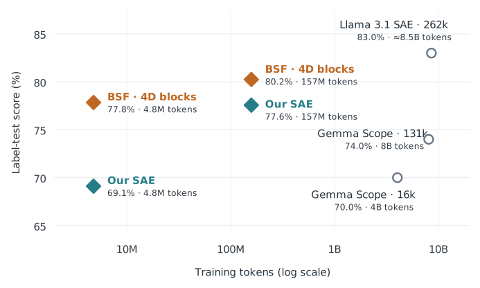
To measure interpretability we first looked to conventional metrics. We first took an LLM which wrote a short description of each given BSF or SAE feature given a sample of its activating examples. A second LLM saw only that description and predicted whether the feature would activate on held-out examples from different documents, with exact predictions scoring perfectly. To compare against open-source SAEs, we report average performance across the full activation range, scored by activation decile. BSFs reached 77.8%, which is comparable to the best open-source SAEs (70.0–83.0%), despite using over 800× fewer training tokens.

BSFs also outperformed an SAE co-trained using the same small number of tokens (69.1%). Both of these results strongly indicate a much greater sample efficiency than SAEs. Furthermore, manual inspection of these results revealed that most incorrect predictions came from the predicting LLM misunderstanding the description or the example’s context (more so than SAEs), not from the feature activating inconsistently. This implies that these interpretability scores for BSFs are, if anything, an understatement.

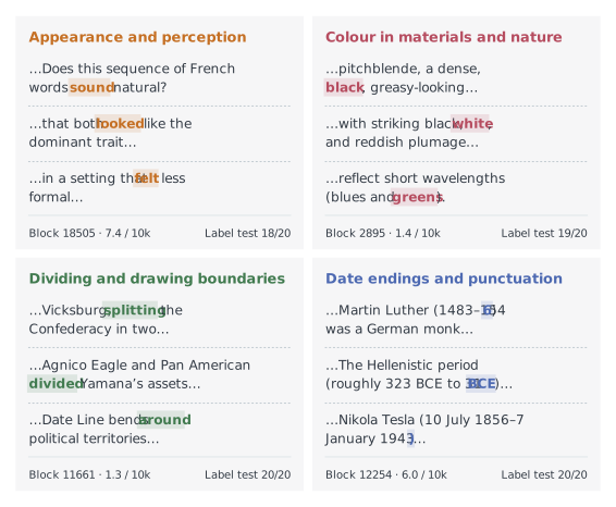
Four-dimensional BSF blocks are shown here combining specialisation with context. One block responds specifically to colour used in scientific description such as black minerals in geology, white feathers in zoology and green light in optics. A date-endings block is likewise notable because its highlighted token always closes a date or a bracket, such as the final digit of “1546”, “BCE” or a closing parenthesis. Earlier work found that language models gather information about the preceding text at these boundary tokens, where sentiment a model’s memory of its context is summarised at commas and other punctuation (Tigges et al.). This block may reflect the same kind of aggregation.

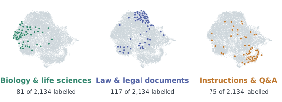
We want to investigate if representing concepts has actually improved. Clustering tests whether features with related meanings have subspaces which sit close to one another. UMAP draws its map from these same decoder directions. Each feature’s nearest neighbours are graphed, and these points are laid out in two dimensions to put neighbours as close together as possible. Below, the labelled blocks are laid out this way.

Loading map…

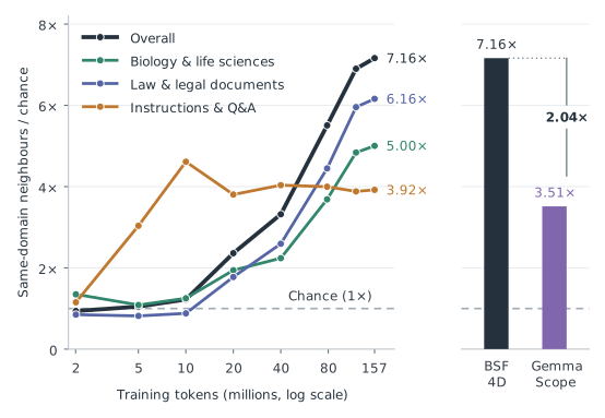
For each feature, it is checked how often its ten nearest labelled neighbours in decoder space shared its domain compared to a random feature. This verifies that the structure is real and not produced purely by UMAP. BSF enrichment rose from near chance early in training to 7.16× chance, compared with 3.51× for domain-matched Gemma Scope.

Each block’s domain label is assigned at the end of training, so the rise in enrichment reflects two processes at once. Related blocks move closer together, and blocks gradually take on the meanings they are eventually labelled with.

The search for known manifolds

Within a BSF block, each token’s activation is a vector. Its length measures how strongly a block is active, and its direction can encode which instance of a concept is present. A manifold appears when these instances form a meaningful geometric arrangement. Manifolds like these are well documented in vision models, where properties such as orientation and colour vary continuously. Similar structures have likewise been reported in language model representations, such as dates around a circle or quantities along a line. Most notably, Engels et al. found that days of the week and months of the year are represented as circles, by grouping related SAE features after training. We looked for known manifolds by testing blocks on predefined token families and checking whether their activation directions showed each family’s natural order.

BSFs are well suited to finding this structure. An SAE learns one-dimensional features, so a circular or continuous concept is broken into many separate latents. The full shape can only be recovered by finding these latents and reassembling them after training. A BSF block is multi-dimensional, so a whole manifold can sit inside a single block, with position on the manifold encoded by activation direction. Months of the year showed this most clearly. Here a well-ordered circle was formed within one BSF block much more clearly than could be matched with SAEs. Days of the week and numbers showed the same advantage, with their natural order preserved more faithfully in BSF blocks. These results indicate that multi-dimensional manifolds as expected are much easier to recover with BSFs than with SAEs. This opens a new direction for interpretability research, in which concepts are studied as continuous geometric structures rather than as collections of isolated features.

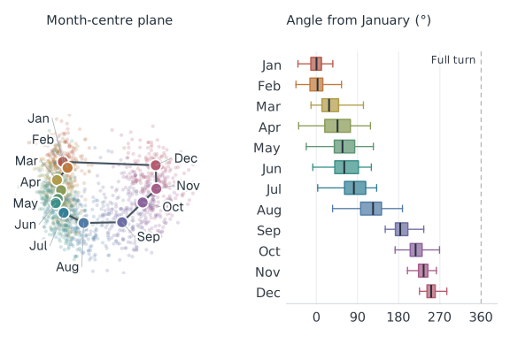
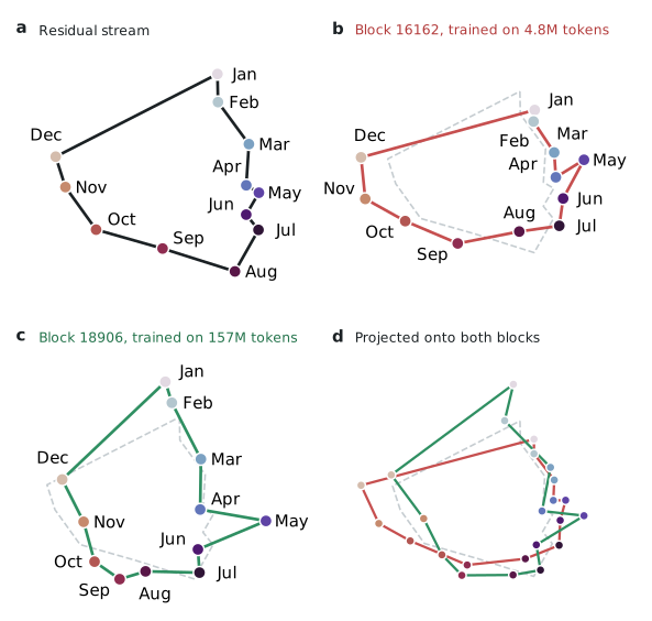
In fact, the aforementioned month circle inside a BSF block is very close to the one that can be read linearly from the residual stream itself. To find this in the residual-stream, we averaged the activations for each month (using their labels) and projected them onto the two directions that best separate the months. This follows the same approach of averaging activations per month as Wurgaft et al., who also rely on known month labels to fit the manifold but leave unsupervised manifold discovery to future work.

That is exactly what the BSF achieves. The blocks never saw the month labels or the order of the months: they were trained, self-supervised, only to reconstruct activations. Even so, when the same activations go through a single block and are averaged by month, they trace the same cycle. Beyond the shape similarities, the block’s four-dimensional subspace contains 36% and 33% of the residual-stream month plane at the two training scales. That is 250 and 231 times what a random four-dimensional subspace would contain, showing this directionality is also preserved.

Projecting the residual-stream month means directly onto each block’s subspace gives back the original loop almost unchanged. The block has not built a new representation of the months. It has found the subspace where the model keeps this representation and carried that structure over linearly into its own coordinates. This mirrors the original BSF paper, where a manifold with known geometry is inserted into the activations and a single block recovers it faithfully. Because this subspace is the model’s own, it could also provide the coordinates for steering along the manifold rather than in a straight line. This can produce more natural changes in the model’s behaviour, without needing any labelled data.

The search for new manifolds

To discover new manifold candidates, we started with each block’s frequently activating tokens. Unlike when we were looking for known manifolds, a family is not specified beforehand. We ranked their geometry against random point sets. An LLM assessed whether the tokens formed a coherent semantic family, and candidates dominated by one document were penalised. We are looking for meaningful lines, rings and other low-dimensional structures. These suggest that a block captures relationships within a concept, beyond detecting its presence.

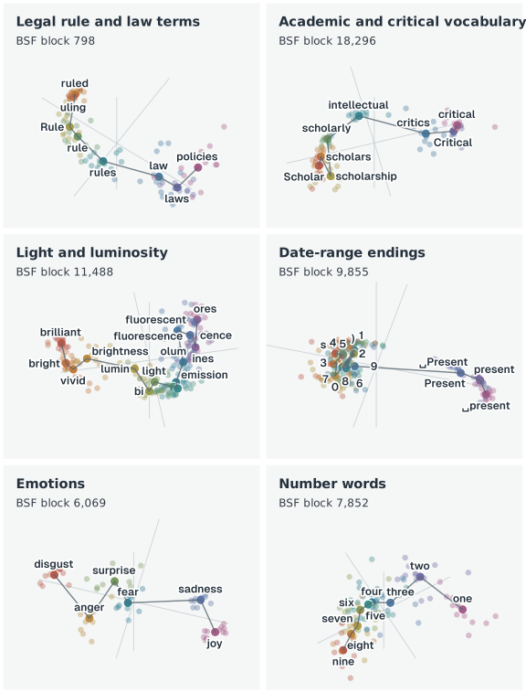
As seen, the date block separates a compact group of digits from “present” variants, potentially distinguishing fixed from open-ended dates. Legal and academic terms form related groups, progressing from rules towards laws and policies. Intellect is also categorised through scholarship towards critical vocabulary. Emotions show a broad ordering, although nearby joy and sadness make its meaning less obvious. These arrangements suggest that a block could preserve a shared concept while using internal directions to encode subgroups and relationships, very similarly to how the month block distinguishes individual months within a common calendar representation.

Appendix: hallucination detection

A.1 Naïve hallucination probes

We look to see if dense probes can be surpassed for hallucination detections using BSFs. A probe trained simply only on the norms of the most active BSF blocks on hallucinations did not match the performance of dense linear probes. This is likely because BSFs have a high reconstruction loss, above that of SAEs. SAEs instead reconstruct the model’s activations closely enough that probes built on them can almost match dense linear probes using all features. BSFs lose some of the information these probes rely on.

We therefore looked inside these blocks at the directions of their activations, as we did for the manifolds. In the months block, for example, one direction indicates that a month is present. Three further directions then arrange the months on a circle, so that January occupies its own position.

Hallucination appears to follow a similar structure. Blocks associated with hallucination carry a clearer hallucination direction, but it sits in the block’s less dominant directions. This matches concurrent work on SAEs and linear probes. Probes trained to separate hallucinated tokens from all other tokens reach a very high AUROC, but much of that performance comes from separating tokens that make a claim from filler tokens. When the probe is trained and evaluated only on claim tokens, it detects hallucinations with a higher AUROC.

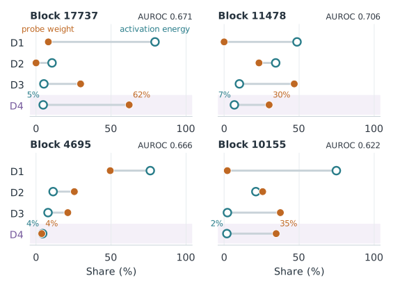
BSF blocks show a matching pattern. Their dominant directions appear to encode the fact that a claim is being made, and the hallucination signal sits alongside these dominant directions. This is intuitive: a hallucination can only occur where a claim is being made. The model may represent it as a variation within its representation of claims, just as a particular month is a position within the representation of months.

We describe this as latching. Rather than forming a block of its own, the hallucination signal attaches to an existing dominant feature, here the claim direction. It can then develop alongside it, expressed only when that feature is active. Latching may also help training. Low-energy concepts, which explain little of the activation variance, are easily overlooked by a reconstruction objective. They may never be given a block of their own, something SAEs are very prone to. By attaching to a dominant feature, such concepts can be learned alongside a direction the dictionary already prioritises. This brings forward subtle but important signals like hallucination that would otherwise be lost.

A.2 Latching mechanism

A simple model explains why BSFs captures hallucinations better than SAEs. A factual claim is a strong direction $\mathbf{f}$ in activation space, with amplitude $A$. A hallucinated claim is the same claim tilted slightly toward a second direction $\mathbf{g}$. This is by a small relative amount $\varepsilon \ll 1$, which is the model’s only free parameter (3). Claims occur on a fraction $p$ of tokens, and a fraction $q$ claims are hallucinated. Hallucination never occurs without a claim for this case.

$$(3)\quad \mathbf{x} = c\,A\,(\mathbf{f} + y\,\varepsilon\,\mathbf{g}) + \mathbf{n} \qquad c \sim \mathrm{Bern}(p) \quad y \sim c \cdot \mathrm{Bern}(q) \quad \varepsilon \ll 1$$

The tilt is too weak to earn an SAE latent of its own. Hence, the SAE folds it into the claim latent, where it survives only as a second-order effect of size $q\varepsilon^2$. A BSF block spanning $\mathbf{f}$ and $\mathbf{g}$ is selected because the claim is strong, and it carries the tilt directly. This is at first order $\varepsilon$, as its second coordinate. Let $\rho = A/\sigma$ be the claim’s signal-to-noise ratio, where $\sigma$ is the noise scale. A hallucination probe on the block has a signal-to-noise ratio $1/(q\varepsilon)$ times higher than one on the SAE (4).

$$(4)\quad \mathrm{SNR}_{\text{BSF}} = \varepsilon\,\rho \qquad \mathrm{SNR}_{\text{SAE}} = q\,\varepsilon^2 \rho \qquad \frac{\mathrm{SNR}_{\text{BSF}}}{\mathrm{SNR}_{\text{SAE}}} = \frac{1}{q\,\varepsilon}$$

Our measurements largely match this picture. We measured the tilt directly in the four Qwen3.8-27B blocks used by the top-K hallucination probe (17737, 11478, 4695 and 10155). In each block, the claim direction $\mathbf{f}$ is the mean code of verified claims, and $\varepsilon$ is the component of the hallucinated claims’ mean perpendicular to $\mathbf{f}$. The tilt’s direction is fitted on half of the answers and $\varepsilon$ is measured on the other half. The tilt is small, as the model assumes: 3.0–11.4° ($\varepsilon = 0.05$–$0.20$). It lies in the blocks’ weaker directions, almost perpendicular to the claim’s main one. Substituting these values and the measured hallucination share ($q = 0.31$–$0.39$) into (4) gives the block up to 62× signal-to-noise advantage over an SAE that absorbs the tilt.

A.3 Informed hallucination probes

Group lasso trains a logistic-regression probe, but with the extra penalty of the sum of the norm of each block’s weight vector. As the penalty is relaxed, whole blocks switch on one at a time. The probe therefore learns jointly which blocks to use and which direction within each block to read, and it favours blocks that work well together over blocks that score well individually.

With four blocks, the probe reaches a test AUROC of 0.781 for Not Supported tokens against all others. That beats every other way of choosing four units: direction-aware ranking (0.737), iterative pruning (0.743), activation-strength ranking (0.637), the four best SAE latents (0.730) and the four best residual-stream dimensions (0.746). The probe still scores 0.781 when each block is reduced to the single number it reads, so the comparison is fair. The gap widens on the harder task of telling true claims from false ones. There the lasso blocks score 0.593, residual dimensions 0.528, and SAE latents 0.494 (as good as chance).

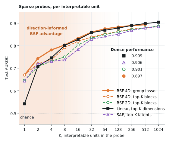
The four blocks the group lasso selects (17737, 12013, 11478 and 10155) are readable. They fire on named entities that open list items, on approximate quantities (“roughly 20–30%”), on paragraph boundaries, and on proper names in citations. Much of the 0.781 therefore comes from finding claims at all. Separating true from false claims is much harder.

A hallucinated claim activates the same block as a faithful one, but its code is tilted slightly towards a direction that carries little of the block’s energy. The lasso finds these directions on its own. In the named-entity block (17737), the probe’s weight lies along the fourth principal axis, which carries only 4.4% of the block’s energy. In the citation-name block (10155), it lies along the second axis, which carries 1.8%.

To test this, we split each four-dimensional block into its dominant direction (the principal axis carrying most of its energy) and the remaining three dimensions. Keeping only the dominant direction is roughly what an SAE latent does: it records how strongly the feature is active and nothing else. Doing so drops true-vs-false performance to chance (0.516, against 0.593 for the full blocks). Keeping only the remaining three dimensions, and so discarding most of the block’s energy, costs nothing (0.597). The information needed to tell a true claim from a false one sits almost entirely in directions a one-dimensional latent cannot represent.

These tilts are not specific to each block. They align closely with the residual stream’s global difference between Not Supported and Supported tokens (median cosine 0.91 across 84 blocks). A single direction assembled from them reaches an AUROC of 0.719 on its own, close in performance to a full 5,120-dimensional linear probe (0.746). The blocks localise a global hallucination signal into the quiet subspaces of claim-related features.

Although BSFs here have shown a new level of interpretability for hallucination, their performance still does not exceed that of a linear probe across all residual stream dimensions. However, they showed improved performance under sparse constraints and distilled hallucination signals alongside interpretable claim blocks.

Concluding remarks

Feature splitting can still scatter one concept across several blocks, while dead blocks leave capacity unused. Variable block sizes for BSFs could address both. Fragments of one feature can be merged, we can split blocks that mix distinct concepts, and can move capacity to features that need more room.

BSFs look like a promising step beyond SAEs. They outperform SAE latents at the same budget, and by keeping a small subspace for each concept they preserve structure that SAEs throw away. That structure includes continuous variables such as hue or orientation, and subtle signals such as the hallucination tilt found here. Studying how activity moves within a block, not just whether a feature fires, could reveal even more about how models represent and transform concepts in ways SAEs have so far left hidden.