4 August 2026Benedict Mullins

Manifold Destiny

Every token in a transformer gets one vector, which travels the length of the model. Attention heads read from it, MLPs write back into it, and nothing else carries information from one layer to the next. Everything the model knows about that token has to fit inside it. This vector is the residual stream, and in Gemma 4 31B it holds 5,376 numbers.

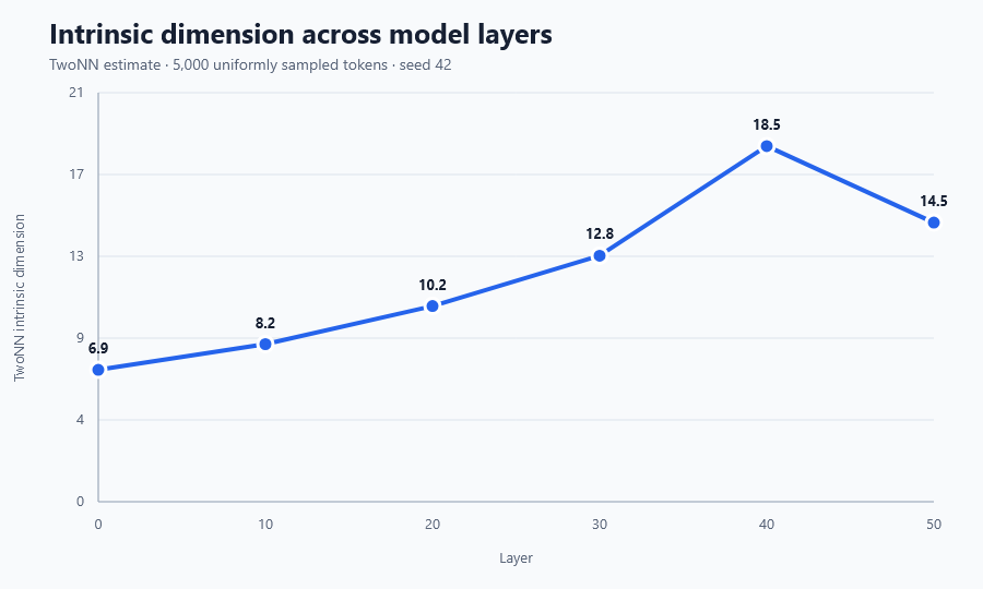
You might expect the model to need all of them. Measured locally, however, the data to attend to a single prompt has between 7 and 19 degrees of freedom: at most a third of one percent of the space.

The Manifold Hypothesis

Suppose you have some extremely high dimensional data taken from the real world, such as the spatial coordinates of a large set of sensors measuring a mechanical system, or a dataset of images of animals. The Manifold Hypothesis states that since it was taken from the real world, it will not actually fully utilise all of those dimensions. Instead there will exist some latent manifold embedded within that space that the data really lies on.

What is an intrinsic dimension?

The classic example is a Swiss roll: a flat sheet curled through three dimensions. Its extrinsic dimension is three. Its intrinsic dimension, the number of degrees of freedom to move along the sheet, is two.

A Swiss roll: a two-dimensional sheet with an extrinsic dimension of three. twoNN recovers the intrinsic dimension of two; PCA, which cannot see past the curvature, reads three. Drag to rotate.

The standard tool to measure intrinsic dimension is principal component analysis, PCA. PCA looks for flat subspaces, so every curve counts as an extra dimension. PCA finds the Swiss roll three-dimensional. In contrast, TwoNN is local and nonlinear. For each point it takes the distances to the nearest and second-nearest neighbours, and the ratio of the two depends only on the intrinsic dimension, which it reads off the slope of a log-log fit. On the Swiss roll it returns two.

What we measured

We ran 237 prompts from LongFact through Gemma 4 31B. Each completion was around a thousand tokens, so the dataset came to roughly a quarter of a million tokens in total. We measured the hidden state at layers 0, 10, 20, 30, 40 and 50.

Tokens from the same completion are typically similar, which will skew a nearest-neighbour estimate. So rather than use every token, we instead took a random sample of 5,000 tokens spread uniformly across the answers.

Line chart of the TwoNN intrinsic dimension estimate across layers 0 to 50 of Gemma 4 31B: 6.9, 8.2, 10.2, 12.8, 18.5 and 14.5. — TwoNN intrinsic dimension by layer.

To check the shape, we ran a second estimator over the same data. L2N2 is from the same family as TwoNN and it also measures dimension from the ratios of nearest-neighbour distances. However, TwoNN needs the data to be locally uniform whereas L2N2 does not.

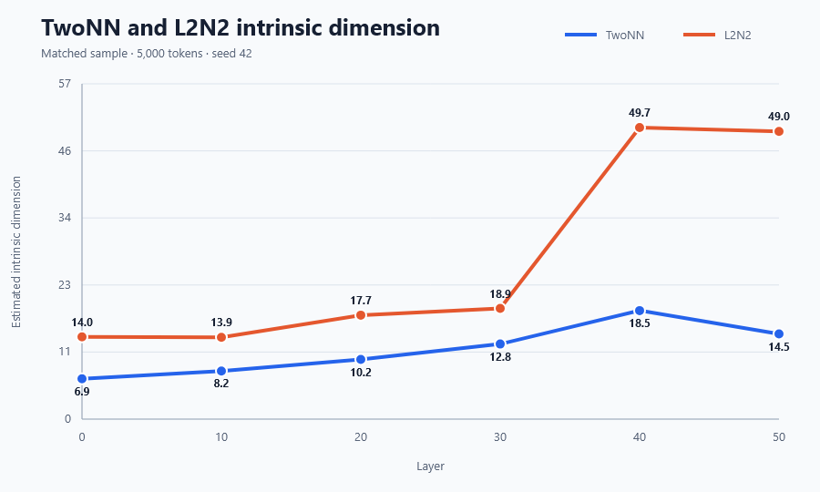
Line chart comparing TwoNN and L2N2 intrinsic dimension estimates across layers. L2N2 reads 14.0, 13.9, 17.7, 18.9, 49.7 and 49.0; TwoNN reads 6.9, 8.2, 10.2, 12.8, 18.5 and 14.5. — TwoNN vs L2N2.

The shape is by no means identical, but both L2N2 and TwoNN peak at layer 40. While L2N2 does read higher at every layer, it is important to keep this in context. L2N2 also tells us that 99% of the residual stream is apparently unused, at least locally.

What are these dimensions doing?

To see what varies, we mapped layer 30 with Isomap, which works to flatten a manifold while keeping distances measured along its surface. We ran 20,000 prompts through it, averaging each prompt's token vectors into a single point.

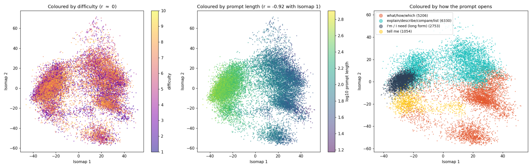
Three Isomap projections of layer 30, coloured by prompt difficulty, by prompt length, and by how the prompt opens. — Layer 30, mapped with Isomap.

The horizontal axis tracks prompt length (r = −0.92). Long prompts, mostly opening "I'm" or "I need", form a dense cluster on the left averaging 311 characters. Everything right of centre averages under 85.

The rest of the map groups prompts by how they open. Questions starting "what", "how" or "which" gather in one region, instructions to explain, describe, compare or list in another, and "tell me" requests in a third. The model was never told about these categories. It sorted prompts by sentence structure on its own.

It's worth noting that the topic seems to have no effect. For example, twenty prompts about the Roman Empire land all over the map, no closer to each other than twenty picked at random. Difficulty also has no meaningful effect (r = 0.004).

So what?

The residual stream is supposed to be dense. Locally, the model uses a small fraction of its freedom to answer any given prompt and still works. If the stream truly is sparse, we could use some smaller dimensional manifold projection to understand what the model is doing, which makes interpretability far more tractable than the extrinsic dimension suggests.

There are still a lot of questions left unanswered. Why does it peak where it does (Ansuini et al.; Valeriani et al.)? Does an untrained model look the same? Does the geometry change when the model is wrong, or during the course of a conversation?

There are also some larger questions raised by these findings. If the local structure is so small, why do we need so many dimensions? Would a smaller model perform just as well as a large one on a specific area and, therefore, would several smaller specialised models beat one general one?

Appendix: comparing four dimensionality reduction algorithms

All four ran on the same 500-token sample, one token drawn from each archive per round, reduced to 200 PCA components first. Trustworthiness scores how well each preserves local neighbourhoods after projection, so it measures distortion, not correctness: a high score means points that were close before are still close, nothing more.

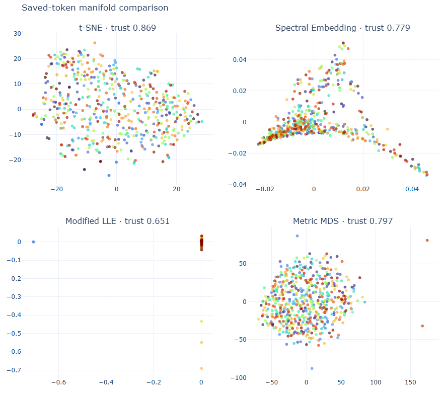
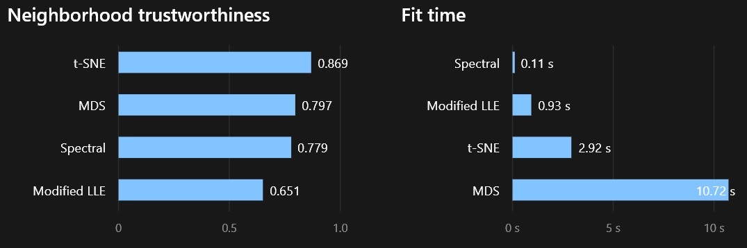
Four scatter plots of the same token sample projected by t-SNE, spectral embedding, modified LLE and metric MDS.

Bar charts of neighbourhood trustworthiness (t-SNE 0.869, MDS 0.797, spectral 0.779, modified LLE 0.651) and fit time (spectral 0.11 s, modified LLE 0.93 s, t-SNE 2.92 s, MDS 10.72 s). — Trustworthiness and fit time.

t-SNE. Points are treated as samples from a probability distribution, and the Kullback-Leibler divergence between the high and low dimensional distributions is minimised. Best trustworthiness of the four, third fastest. Scikit-learn documents it as a visualisation tool rather than an analysis one, so treat the output as a picture rather than a measurement.

Metric MDS. Aims to reproduce pairwise distances directly; metric MDS preserves distance magnitude, non-metric MDS preserves only the ordering. Second best trustworthiness, and much the slowest.

Spectral embedding. Builds a neighbourhood graph and uses the eigenvectors of its Laplacian. Fastest by a wide margin and good on curved or disconnected structure. New points can't be transformed directly and need a Nyström extension, which limits it where activations arrive continuously. The embedding looked visibly distorted, yet scored close to metric MDS on trustworthiness.

Modified LLE. Preserves local neighbourhood geometry. LLE fits a weight vector per neighbourhood and optimises the set for projection; modified LLE uses several linearly independent weight vectors per neighbourhood rather than one. Worst trustworthiness, middling runtime, and spectral embedding beats it on both, so there's no regime where it's the right choice.