
Quantisation and surrogate probes
Motivation
It is known that quantisation can negatively affect a model’s output quality. However, there is evidence that suggests that quantisation does not meaningfully affect the internal activations of the model during the prefill stage, the cheap and efficient part of inference that our probes read from.
We care because Telluvian's work is largely based on surrogate model interpretability. In short, this is when a closed model's transcript is replayed through an open-weight ‘surrogate’ model. Linear probes are then used to detect behaviours in the surrogate that then generalise to the original closed weight model. Quantising the surrogate would make this process cheaper and possibly faster. The purpose of this experiment is to test whether quantising the surrogate affects probe performance.
Some of our earlier work by Ben Mullins found that quantisation costs our probes nothing in terms of performance and that NVFP4 cuts GPU time by around 40%. That matched what we'd seen in production, but it was a quick check on one layer and one seed. We wanted a result we could defend. So I measured probe performance across a range of layers and quantisations, on two datasets, against a range of benchmarks.
Headline result: From 16 down to about 4 bits, no meaningful performance degradation is present. Below that the probes start to degrade meaningfully.
Method
We used two datasets with different behaviours:
- Coding Agent Misalignment (CAM): 2,318 coding-agent sessions, with tokens labelled where GPT-5.4 flagged the agent as overconfident and lazy. This dataset also included a number of other LLM judges; however, we elected to use a single model as a judge to provide a consistent behaviour for the probes to learn. GPT-5.4 was chosen as it had the highest positive rate. This decision was practical for our purposes but means the probes have no practical use beyond aping GPT-5.4 reactions to CAM.
- 12,000 question-and-answer records from GPT-5.6-Luna, with positive tokens labelled where GPT-5.6-Terra marked a claim as unsupported.
Both use LLM-judge labels, so the probes primarily learn to imitate a judge rather than detect the behaviour itself. That's not a problem in our case. Our primary concern is using a consistent dataset rather than measuring any specific semantics. Full details of the datasets and method are in the appendix.
We first trained probes on the unquantised (bf16) Qwen3.8-27B, as a baseline. We then used each quantised version to answer two questions:
- Reused: do the original probes still work on the quantised model's hidden states? This is what we'd actually deploy.
- Retrained: if we train fresh probes on the quantised states, is the information still there?
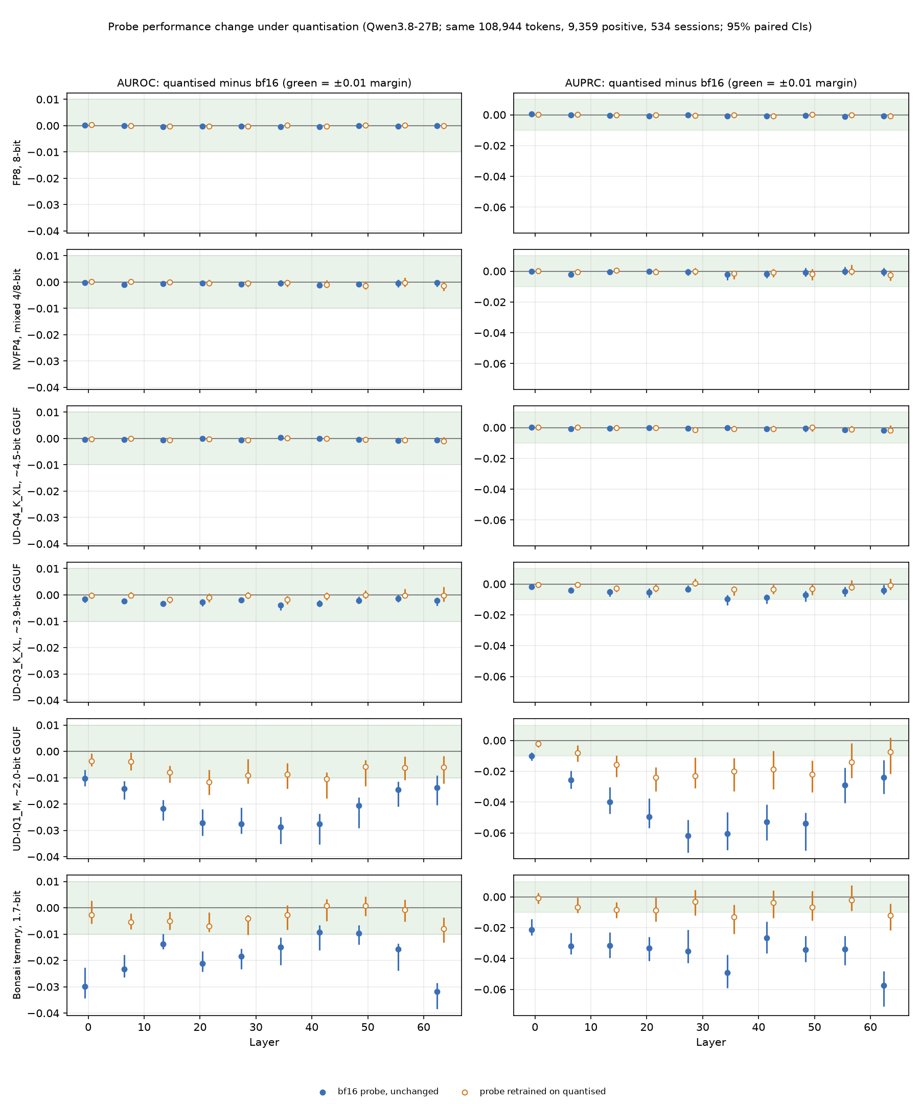
We scored both on AUROC and AUPRC at 10 layers. A model counted as equivalent to bf16 if the 95% confidence interval on the difference sat inside ±0.01. We fixed that margin before running anything; it's about five times the variation we get from retraining a probe with a different seed.
We also measured ‘drift’ as the size of the change in each hidden state relative to its original size, where 0 means no change. Cosine and L2 drift were used at various points.
We used the following models as part of the study.
| Name | Checkpoint | Bits/weight | Engine |
|---|---|---|---|
| bf16 | Qwen/Qwen3.8-27B @1d4bf0f2 | 16 | vLLM |
| FP8 | Qwen3.8-27B-FP8 @017b9c7a | 8 | vLLM |
| NVFP4 | NVIDIA NVFP4, mixed 4/8 @482ca0f3 | ~4.5 nominal (~6.5 by file size) | vLLM, CUTLASS linear backend |
| Q4_K_XL | unsloth/Qwen3.8-27B-GGUF UD-Q4_K_XL | ~4.5 nominal (~5.2 by file size) | llama.cpp |
| Q3_K_XL | same repo, UD-Q3_K_XL | ~3.9 | llama.cpp |
| IQ1_M | same repo, UD-IQ1_M | ~2.0 (not 1-bit, despite the name) | llama.cpp |
| Ternary Bonsai | prism-ml/Ternary-Bonsai-2-27B-gguf @b072e1d3 PTQ1_0 | 1.7 | llama.cpp |
| Bonsai-27B Q1_0 | prism-ml/Bonsai-27B-gguf @f10afb35 (base Qwen3.6-27B @6a9e13bd) | ~1.1 | llama.cpp |
NVFP4 and Q4_K_XL are labelled by nominal format in the figures and are higher by file size, so treat the bits axis as approximate. A note on engine control. bf16 in llama.cpp and in vLLM differ by at most 0.0003 in probe metrics, with hidden-state cosine ≥ 0.995 at every layer. GGUF differences are therefore due to quantisation rather than the engine.
Regarding expectations, quantisation is generally considered lossless and stable down to approximately 4 bits. Therefore I was expecting this to be a threshold at which things may start to break down. I was unsure as to how different versions of the same quantisation (i.e. NVFP4 and UD-Q4_K_XL) would perform, my expectation was that they would be more different than reasonable.
Baselines
As well as comparing to the unquantised model, we decided to test against a number of additional benchmarks. The rationale was that if a probe only picked up surface wording, any quantised model would preserve it and the test would tell us nothing. So we first compared the bf16 probe with text-only baselines: TF-IDF, Qwen3 embeddings, BM25 retrieval, and a model that sees only token position and transcript length. How each baseline works, with full results, is in the appendix.
The linear probe comfortably outperformed the benchmarks. At layer 49 it beats TF-IDF (the strongest baseline) by 0.19 AUPRC on CAM and 0.26 on Luna. Position and length are close to chance. Therefore, we can say with confidence that the probe is reading something from the model's internal state that can't be gleaned from just the input/output text.

Results
Down to 4 bits
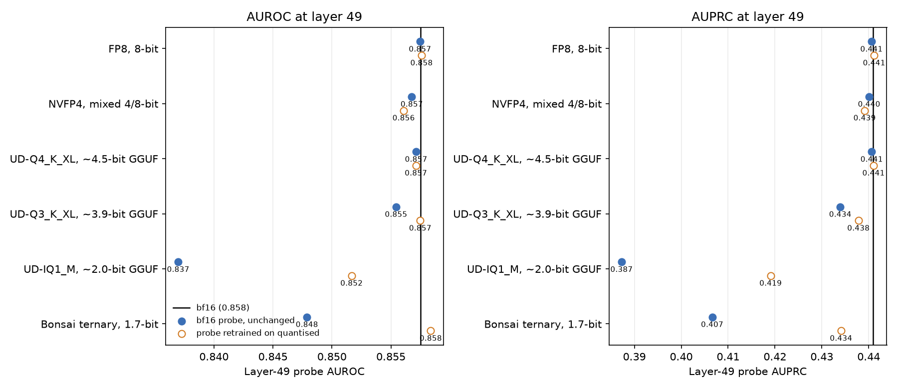
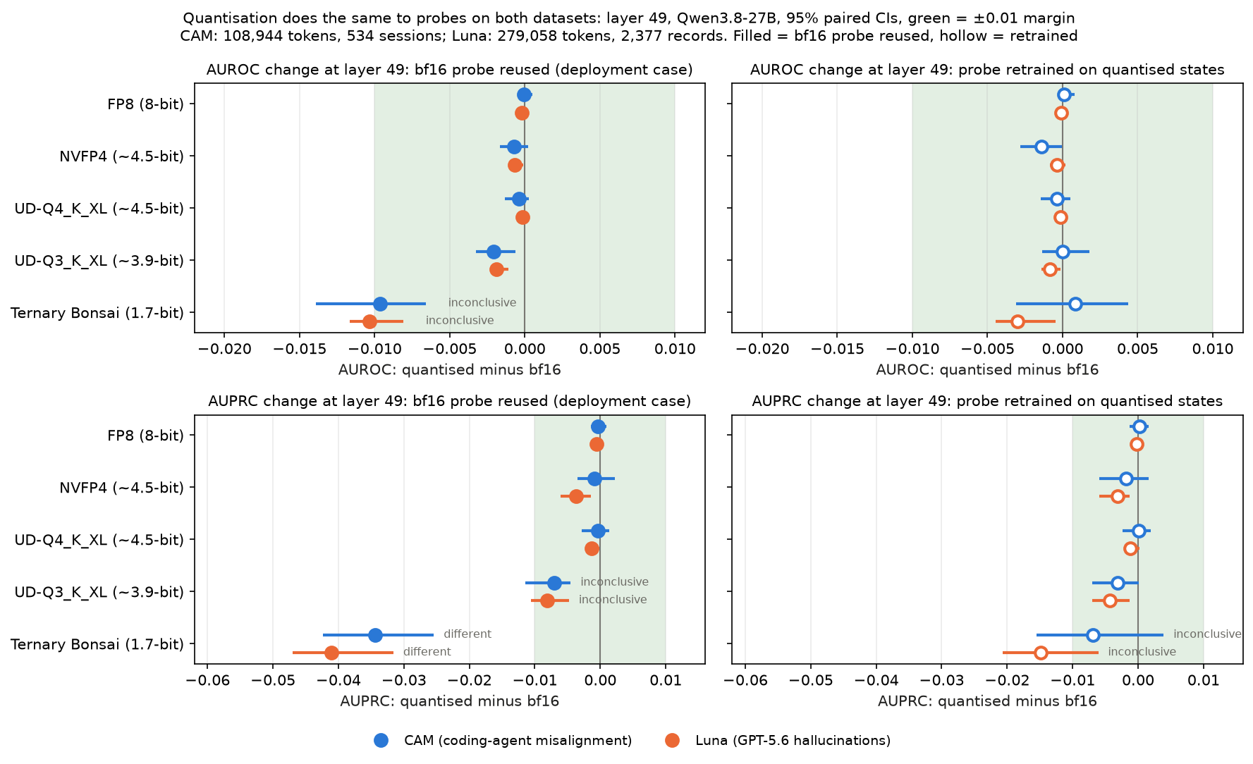
FP8, NVFP4 and Q4_K_XL were equivalent to bf16 at every layer, on both metrics and both datasets, whether we reused the probes or retrained them. The largest difference anywhere was 0.004, which is comfortably less than our equivalence margin of 0.01.
| Model | Bits | Prefill speed vs bf16 | Largest change, reused probe (CAM / Luna) |
|---|---|---|---|
| FP8 | 8 | 1.31× | 0.0012 / 0.0012 |
| NVFP4 | ~4.5 | 1.54× | 0.0023 / 0.0036 |
| Q4_K_XL | ~4.5 | 0.89× (llama.cpp) | 0.0019 / 0.0013 |
NVFP4 has the fastest throughput, at approximately 1.5 times bf16 prefill speed on both datasets.
Below 4 bits
Q3_K_XL (~3.9 bits) is marginally smaller than NVFP4 and Q4_K_XL and shows increased degradation as expected. It loses about 0.007 AUPRC at layer 49 on both datasets. It is worth noting that this is still within the equivalence margin. A retrained probe recovers essentially all of this loss.
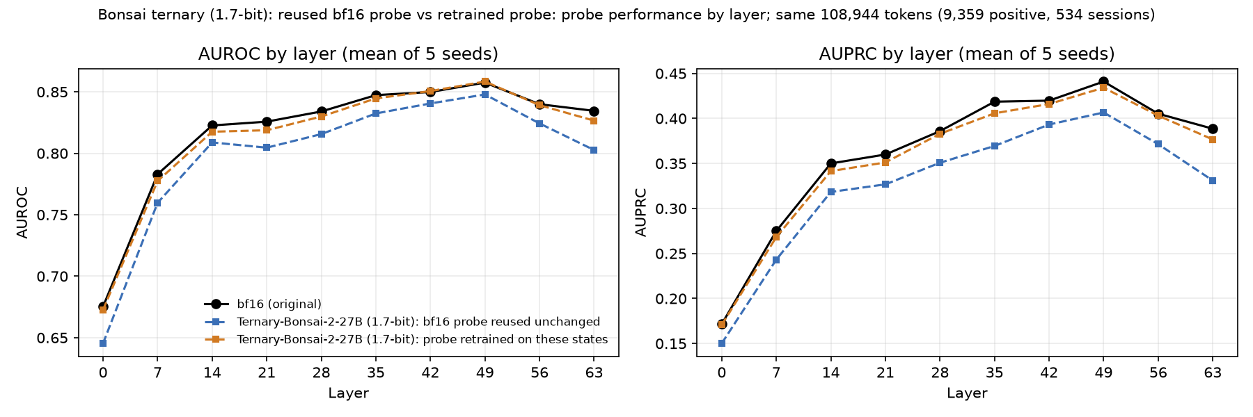
By around 2 bits the performance loss is clear. IQ1_M's reused probe loses 0.054 AUPRC at layer 49 and falls significantly outside the margin. Retraining helps, but still leaves it about 0.02 down in the deeper layers. A true 1-bit model, Bonsai-27B Q1_0, is worse still: the reused probe loses 0.115 AUPRC, and retraining recovers about 85% of that.
| Model | Bits | AUPRC change at layer 49, reused (CAM / Luna) | Retrained (CAM / Luna) |
|---|---|---|---|
| Q3_K_XL | ~3.9 | −0.007 / −0.008 | −0.003 / −0.004 |
| IQ1_M | ~2.0 | −0.054 / not run | −0.022 / not run |
| Ternary Bonsai | 1.7 | −0.034 / −0.041 | −0.007 / −0.015 |
| Bonsai-27B Q1_0 | ~1.1 | −0.115 / not run | −0.018 / not run |
Please note that Bonsai-27B Q1_0 is built on Qwen3.6 rather than Qwen3.8, so it is compared with Qwen3.6 instead (see the appendix).
The only model to buck the trend is IQ1_M. It has more bits per weight than ternary Bonsai (2.0 against 1.7) but exhibits more performance loss. This is with both reused and retrained probes.
It is worth noting that both datasets agreed model by model throughout.
Drift
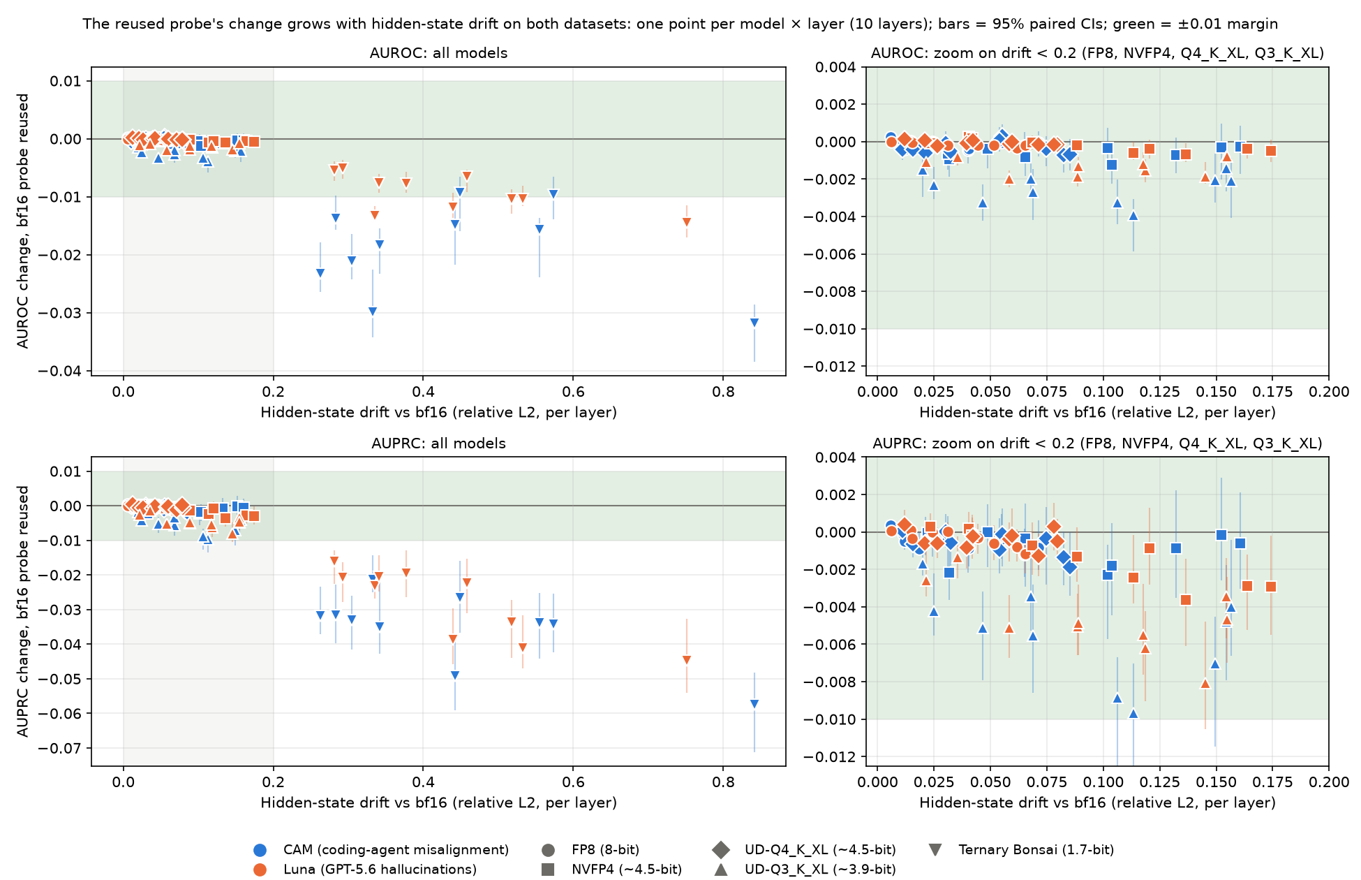
A potential alternative measurement of probe degradation was drift. A probe is just measuring the hidden state and so if the state barely moves, the probe's output shouldn't either. After the first few models it looked like that might work. However, the next few results destroyed that correlation. Q3_K_XL drifts about as far as NVFP4 (0.15 at layer 49), but shows notably worse performance. IQ1_M drifts less than ternary Bonsai (0.47 against 0.57) but loses more.
Probe performance and drift are clearly correlated, but drift isn't reliable enough to use on its own. Taking it at face value, I would speculate that drift depends heavily on the specific quantisation scheme. Cosine drift is especially poor: it reported 0.996 similarity at a layer where the probe lost AUPRC.
Why do low-bit models degrade?
We wanted to know if the performance loss was because low-bit quantisation destroys what the probe reads or if it just moves it. To test this, we fit a linear map from the ternary Bonsai's hidden states back to bf16's, then ran the original bf16 probe on the mapped states. The Luna Hallucinations dataset was used.
| Layer | bf16 | Reused | Per-dimension rescale | Linear map (eval R²) | Linear map recovers | Cosine raw → standardised |
|---|---|---|---|---|---|---|
| 0 | 0.273 | 0.250 | 0.250 | 0.268 (0.94) | 75% | 0.996 → 0.813 |
| 7 | 0.305 | 0.289 | 0.290 | 0.305 (0.81) | 99% | 0.985 → 0.849 |
| 21 | 0.358 | 0.337 | 0.338 | 0.357 (0.80) | 97% | 0.953 → 0.832 |
| 35 | 0.409 | 0.371 | 0.373 | 0.400 (0.77) | 75% | 0.901 → 0.780 |
| 49 | 0.451 | 0.410 | 0.414 | 0.435 (0.78) | 61% | 0.845 → 0.768 |
| 63 | 0.417 | 0.372 | 0.374 | 0.396 (0.76) | 51% | 0.768 → 0.741 |
At layers 7 and 21, the map recovers 97–99% of the lost AUPRC, about as much as retraining a probe. By contrast, rescaling each dimension separately recovers at most 10%. From this, we can conclude that the quantisation is mixing dimensions together, and so a simple rescale can't undo it. Deeper in the model the map recovers less (75% at layer 35, falling to 51% at layer 63), so at least some of the information there is truly lost.
Conclusions
- Down to Q4_K_XL and NVFP4 (~4.5 bits nominal), quantisation has no measurable effect on probe performance at any layer, for reused or retrained probes, on two independent datasets. Every effect is at least 2.5× inside the margin.
- Q3_K_XL (~3.9 bits) is the first format to move a reused probe (L49 AUPRC −0.007 on CAM, −0.008 on Luna). Retraining removes the effect.
- At ~2 bits and below, reused probes degrade significantly and retraining recovers only part of the loss.
- The damage depends on the kind of distortion, not solely on bits or drift.
Limitations
- Only one surrogate family (Qwen) was used.
- There was a very low positive rate for both datasets. As such token rows were sampled with enriched positives.
- Bonsai-27B Q1_0 rests on a different base model, with an off-template reference.
Next steps
NVFP4 in production. NVFP4 matched bf16 on both datasets while running about 1.5× faster, so the next step is to test it in production. This could raise surrogate throughput and cut serving cost without retraining any probes.
Combining this with other interpretability techniques. We'd like to combine this activation measurement scheme with other interpretability techniques, such as the J-space. This may be particularly useful for improving model selection in Gallery.