
Code for this post → github.com/telluvian/twonn
How many intrinsic dimensions does your data really have? Large datasets have a high-dimensional space, but this number of ‘extrinsic’ dimensions often isn’t indicative of the dataset’s underlying complexity. For example, a Swiss roll is a two-dimensional sheet curled through three-dimensional space: extrinsic dimension of three, effective degrees of freedom of two. That smaller number, the effective degrees of freedom, is also called the ‘intrinsic dimension’; it sets how far the data compresses and how many variables a model needs. TwoNN, introduced by Facco, d’Errico, Rodriguez and Laio in 2017, is a mathematical method to estimate the intrinsic dimensionality from measurements of the two nearest neighbours of each point.
Why is intrinsic dimensionality so hard to measure?
The standard tool is principal component analysis (PCA). In short, PCA resolves the data into orthogonal directions of variance and counts how many carry significant weight. However, PCA is only exact when the manifold is a linear subspace, which maps poorly onto real data. For example, curvature reads as extra dimensions: a curved two-dimensional sheet like our Swiss roll would be read as three-dimensional by PCA. There are a number of other issues too, non-uniform density and feature scaling shift the variances and blur the PCA count.
By contrast, twoNN is local and nonlinear. Using only the first two neighbour distances of each point, it measures the dimension of the manifold rather than of the subspace enclosing it, needs no variance threshold, and cancels density through the neighbour ratio. On the Swiss roll, it returns two where PCA returns three.
How does twoNN work?
For each point, take the distance to its nearest neighbour \(r_1\) and to its second-nearest \(r_2\), and form \(\mu = r_2/r_1\), where \(\mu \geq 1\). Then:
- Compute \(\mu\) for every point.
- Sort ascending; the \(k\)-th value has empirical cumulative probability \(k/N\).
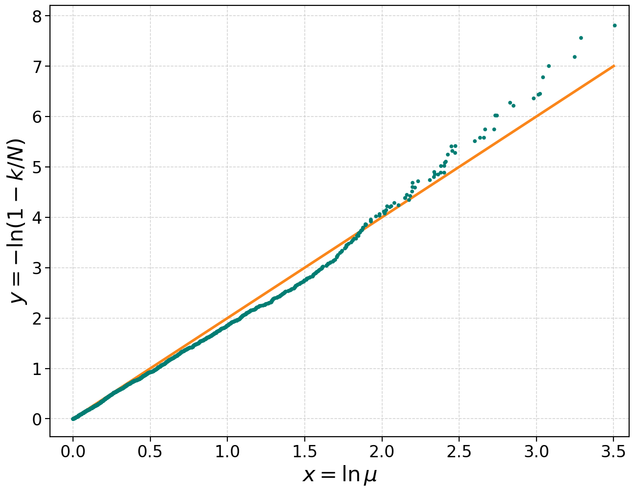
- Plot \(y = -\ln(1 - k/N)\) against \(x = \ln \mu\).
- Fit a line through the origin; its slope is the estimated dimension \(\hat{d} = (\sum xy)/(\sum x^2)\).
As a practical point, heavy tails produce rare, very large \(\mu\) that destabilise the fit, so discarding the largest 10% of values before fitting improves the results. Additionally, by using only two neighbours per point, it runs in near-linearithmic time.
So why does twoNN work?
Fix a point \(x\), with nearest neighbour \(x_1\) at distance \(r_1\) and second-nearest \(x_2\) at distance \(r_2\). Draw the ball of radius \(r_2\) about \(x\): by construction \(x_2\) lies on its boundary and \(x_1\) lies somewhere inside.
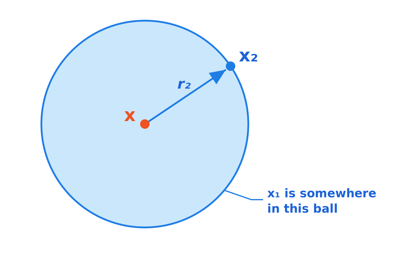
Take \(r_2\) small enough that the density is roughly constant across the ball, the local-uniformity assumption. Then \(x_1\) is uniform within the ball, and its position alone fixes the ratio \(\mu = r_2/r_1\).
Shrink an inner ball to half the radius, \(r_2/2\). Where \(x_1\) falls decides \(\mu\): on the boundary gives \(r_1 = r_2/2\) and \(\mu = 2\); inside gives \(\mu > 2\); outside gives \(\mu < 2\). So \(\mu \geq 2\) is exactly the event that \(x_1\) lands in the inner ball, and under uniformity its probability is the volume ratio. Since volume scales as \(\text{radius}^d\),
\[ P(\mu \geq 2) = P\left(r_1 \leq \frac{r_2}{2}\right) \approx \left(\frac{1}{2}\right)^d = 2^{-d} \]
The radius is the only thing that changed. Replace 2 with any \(a > 1\): an inner ball of radius \(r_2/a\) captures exactly the event \(\mu \geq a\), giving
\[ P(\mu \geq a) \approx \left(\frac{1}{a}\right)^d = a^{-d} \]
That is the tail of \(\mu\), so its cumulative distribution is
\[ F(\mu) = P(\mu' \leq \mu) \approx 1 - \mu^{-d}, \quad \mu \geq 1 \]
From distribution to a straight line
Sort the observed ratios; the \(k\)-th value \(\mu_k\) sits at the empirical quantile \(k/N\), so
\[ \frac{k}{N} \approx 1 - \mu_k^{-d} \]
Rearranging and taking logs,
\[ -\ln\left(1 - \frac{k}{N}\right) \approx d \cdot \ln \mu_k \]
Plot \(y_k = -\ln(1 - k/N)\) against \(x_k = \ln \mu_k\) and the points fall on a line through the origin with slope \(d\). That slope is the estimate.
How does this apply to transformers?
We measured the residual stream intrinsic dimensions for gemma-4-31B-it, taking the residual stream over 100 completions on recall-based prompts at a maximum sequence length of 2048. The stream is 5,376-dimensional, yet the per-layer local intrinsic dimension was measured to be between approximately 4 and 12. That is to say, the structure the model actually uses occupies a thin manifold inside a very large space.
View the underlying data ›
| Layer | Effective dimension |
|---|---|
| 0 | 4.60 |
| 10 | 6.38 |
| 20 | 7.34 |
| 30 | 11.18 |
| 40 | 10.54 |
| 50 | 7.79 |
This surprising result is backed up by existing studies, see Less is More: Local Intrinsic Dimensions of Contextual Language Models for further information. This study applies exactly this twoNN method to contextual token embeddings and finds the same picture: the extrinsic dimension may be hundreds or thousands, whereas the local intrinsic dimension reflects a much lower-dimensional manifold that varies across regions of the space. Their mean local dimensions sit in the same range as our results (around order of 10) across the models they tested: RoBERTa, Llama-3.1-8B, Phi-3.5 and others.
So what?
The effective space really is shockingly small. It’s hard to visualise, but the fact is that a layer that should be thousands of dimensions behaves, locally, like it has only a dozen. You would expect a model this well developed to be using far more of the room available to it, and it straight up isn’t. That gap is unexpected, unexplained, and chronically unexplored. Since the effective part of the model is so much smaller than it looks, it’s also far more tractable to study.
This has opened up a few directions of exciting research:
- Interpretability. A layer with an effective size of around a dozen is suddenly a lot more approachable. Instead of reasoning about thousands of dimensions, we’re instead looking at a small subset of directions that capture what the model is really representing at that point, which makes it far easier to ask what those directions mean. In addition, the smaller size means we may be more able to measure how the manifold reshapes as a model learns, further improving our understanding of the model’s learning process.
- Steering. Once you know the shape of that smaller manifold, you may even be able to start to move within it deliberately. To date, model steering has been an unqualified disappointment. It’s possible that the problem has been an over-focus on the model’s global dimensions rather than a local manifold. If so, working with a low-dimensional surface, rather than the overall high dimensional space, is a much more promising basis for controlled, predictable steering.
- Fine-tuning. The intrinsic size also tells you how much 'space' a task actually needs. It can give us a quantifiable and principled way to measure what a model is thinking and therefore calibrate it better on specific features.
The bottom line is that a surprisingly small intrinsic state space makes the model easier to see into, easier to guide, and easier to adapt. That’s where we’re taking this research next.
Try it yourself → github.com/telluvian/twonn
Further reading
- Facco, E., d’Errico, M., Rodriguez, A. & Laio, A. “Estimating the intrinsic dimension of datasets by a minimal neighborhood information.” Scientific Reports 7, 12140 (2017). Open access (CC BY 4.0).
- Sato, R. “TwoNN Intrinsic Dimension Explained: Python and Visual Illustrations.” Data Processing Club (2025).